The iris dataset is widely renown among machine learning enthusiasts. It contains three species of flowers (setosa, versicolor, virginica) with 4 relative attributes: petal length, petal width, sepal length, sepal width.
What we’re going to do is try to predict the species of flower knowing its attributes.
Today I’ve decided to show how to train one of the most popular models these days: a Decision Tree classifier.
Let’s see how it works.
Decision Tree Classifier
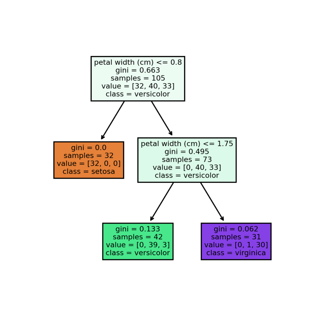
As you can see at each node the tree makes a decision and divides itself into two branches. The nodes which have no more ramifications are called leafs and are used by the model to make the final predictions.
Now you should be wandering: what’s “gini” there? Well, the Gini impurity is the cost function the algorithm will minimize. It’s defined as follows:

Where n is the number of different classes (in this case 3) and 
To be clear, the Gini impurity of the purple leaf is calculated as follows:
^2 - (1/31)^2 - (30/31)^2")
The lower it is, the more accurate the prediction.
Now let’s see the code behind that tree.
from sklearn import datasets
import matplotlib.pyplot as plt
import numpy as np
import pandas as pd
from sklearn.tree import DecisionTreeClassifier, plot_tree
from sklearn.model_selection import train_test_split
from sklearn.metrics import accuracy_score


iris = datasets.load_iris()
X = pd.DataFrame(iris['data'], columns=['sepal length', 'sepal width', 'petal length', 'petal width'])
y = np.array(iris['target'])


X_train, X_test, y_train, y_test = train_test_split(X, y, test_size=0.3, random_state=123)

t_clf = DecisionTreeClassifier(max_depth=2)
t_clf.fit(X_train, y_train)
y_pred = t_clf.predict(X_test)

fn = ['sepal length (cm)', 'sepal width (cm)', 'petal length (cm)', 'petal width (cm)']
cn = ['setosa', 'versicolor', 'virginica']
fig, axes = plt.subplots(nrows=1, ncols=1, figsize=(4, 4), dpi=300)

plot_tree(t_clf, feature_names=fn, class_names=cn, filled=True)
fig.savefig('tree.png')

print(accuracy_score(y_pred, y_test))
So, what I did is at first loading the datasets and creating the training instances (X) and the target variables (y). Obviously I used pandas and numpy, two very important libraries in machine learning.
After that I used the scikit-learn train_test_split function to divide the dataset into a part which will be used for training the model and the other used for testing its predictions on unseen data with a ratio of 7/3. The attribute random_state of train_test_split is only used for reproducibility (by setting it equal to 123 on your own code it will give you the same result as mine).
Then I created the Decision Tree: “max_depth = 2” means there can only be 2 ramifications and prevents an overfitting (meaning the model doesn’t generalize well on unseen data) of the training data. Then the model is trained on the data and makes its predictions.
The part that follows is only a way to reproduce the image you can see above, so you can have your own too.
Finally, I print the ratio of correct predictions out of the total instances and the result is pretty good already: 0.9555555555555556.
Anyway, there are models which are even more powerful than this one, such as the Random Forest Classifier, which is an ensemble method which is made out of many Decision Trees which are trained on different subset of the data to make a very accurate final prediction.
We’ll see them in another article.